LSTM Predict Stock Price | chenoiLab

icon

password

You can find the original code here.

Imagine you are watching a long movie, and LSTM is like your brain. During the viewing process, your brain unconsciously remembers certain key scenes, characters, and plots, and constantly recalls and references this information to understand the story of the movie. LSTM does something similar: when processing data sequences (such as stock prices), it remembers past information and uses it to understand or predict future trends.

Temporal Dependency: LSTM (Long Short-Term Memory) layers are suitable for time series data, such as stock prices, because they can "remember" past information. They are able to capture the temporal dependency in the data, which is crucial for predicting future prices.

Avoiding Vanishing/Exploding Gradient Problems: When dealing with long sequences, regular Recurrent Neural Networks (RNNs) often encounter vanishing or exploding gradient problems. LSTM helps alleviate these issues with its special structure, making it more suitable for handling time series problems.

There are four features in the data (Open, High, Low, Volume) as inputs, and the output is Close. LSTM layer is suitable because it can capture the long-term dependencies in this time series data, as the price of each day may be influenced by the prices of previous days.

The choice of the first LSTM layer in the model is 128 units. Generally, the first layer usually has more units than the second layer to capture more information. return_sequences=True means that the hidden state of each time step in this layer will be passed to the next layer. This is necessary for stacking LSTM layers.

The choice of the second LSTM layer is 64 units. This layer does not return the entire sequence to the next layer because it is followed by a fully connected layer, which expects input from a single sample rather than a sequence.

The subsequent Dense layer is for feature transformation and output prediction. This layer is often used as a hidden layer to capture more non-linear features before the output layer.

Output layer (1 unit): Our goal is to predict the next closing price, so we only need 1 node to output the predicted value.

In this example, we only use "Open", "High", "Low", "Volume" as input features, possible reasons include:

Model Input: In the model training mentioned above, the input data x is composed of "Open", "High", "Low", "Volume". These features contain the daily dynamics of the stock and may be considered useful for predicting the closing price "Close".

Avoiding Data Leakage: We did not use "Close" and "Adj Close" as input features, possibly to avoid data leakage from the future. In theory, when predicting future closing prices, we should not have knowledge of the future closing prices.

Data Download

yf.download: Downloads stock data using the yfinance library.

Date and Time Handling

date.today(): Gets the current date.

strftime: Formats a date into a string.

timedelta: Represents the difference between two dates or times.

Data Processing

data["Date"] = data.index: Moves the date from the index column to a new "Date" column.

data[["Date", "Open", "High", "Low", "Close", "Adj Close", "Volume"]]: Selects a subset of the data.

Data Visualization

go.Figure: Creates a Plotly figure object.

go.Candlestick: Creates a candlestick chart object.

Data Analysis

data.corr(): Calculates the correlation coefficients between columns in a DataFrame.

Building and Training the Neural Network Model

Sequential: A linear stack of layers used for creating a neural network.

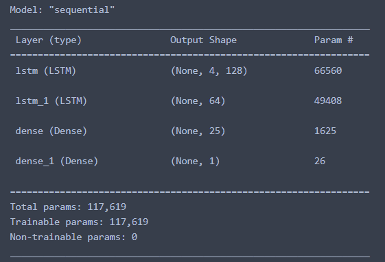
model.summary(): Outputs a summary of the model, including the number of layers and the output dimensions of each layer.

model.compile: Configures the learning process of the model, including specifying the optimizer and loss function.

model.fit: Trains the model on the training set.

In LSTM, each gate (forget gate, input gate, output gate) and the update of the cell state have their own weight matrix and bias vector. Specifically, given an input feature size D and a hidden unit size H, we have the following parameter calculations:

Weight Matrix: There is a weight matrix for each gate, with a size of [D, H]; there is also a weight matrix for the cell state update, with the same size of [D, H]. In total, there are 4 such matrices, so the total number of weight parameters is .

Recurrent Weight Matrix: For each gate and cell state update, we also have a recurrent weight matrix, with a size of [H, H]. So, these parameters add up to .

Bias Vector: Each gate and cell state update has a bias vector with a length of H. In total, there are bias parameters.

Based on the above parameters, the total number of parameters in one LSTM layer is:

Total LSTM params = 4 x (D x H + H^2 + H)

First LSTM layer:

D = 1 (since the number of input features is 1)

H = 128

Second layer LSTM (Note that now D depends on the previous layer's H):

D = 128
H = 64

The calculation of parameters for a Dense layer is relatively simple. Given the number of input nodes N and the number of output nodes M, the number of weight parameters is , and the number of bias parameters is M. In other words:

First Dense Layer:

N = 64
M = 25

Second Dense Layer:

N = 25
M = 1

Total number of parameters for the entire model: 66560 + 49408 + 1625 + 26 = 117619

For tasks like stock price prediction, having too many parameters can sometimes capture noise in the data instead of true trends, which can lead to overfitting.

Considering there are 117,619 parameters, it is important to ensure that you have enough training data. In general, it is desirable for each parameter to correspond to at least a few data points to avoid overfitting.